
Published: . Last updated: .
In late 1865 cows began dying in large numbers in England. This cattle plague was probably caused by the Rinderpest virus. Beef had become a vital part of the economy and so there was concern at the highest level of government. A commission was set up to investigate the epidemic. In February 1866, Robert Lowe, a Member of Parliament on this commission, made a gloomy prediction:
If we do not get the disease under by the middle of April, prepare yourself for a calamity beyond all calculation. You have seen the thing in its infancy. Wait and you will see the averages, which have been thousands, grow to tens of thousands, for there is no reason why the same terrible law of increase which has prevailed hitherto should not prevail henceforth. (Brownlee, BMJ, 14 Aug 1915, p. 251)
William Farr was an epidemiologist who had in 1840 shown that the distribution of smallpox deaths was approximated by a normal curve. Actually the term "normal" wasn't part of statistical terminology until several decades later. Farr wrote: "The rates vary with the density of the population, the numbers susceptible of attack, the mortality, and the accidental circumstances; so that to obtain the mean rates applicable to the whole population, or to any portion of the population, several epidemics should be investigated. It appears probable, however, that the smallpox increases at an accelerated and then a retarded rate; that it declines first at a slightly accelerated, and at a rapidly accelerated, and lastly at a retarded rate, until the disease attains the minimum intensity, and remains stationary." That's indeed a description of what we today call a normal curve.
In 1866 Farr wrote a letter to the Daily News, a newspaper started 20 years earlier by Charles Dickens. Explaining why things were not quite as awful as Lowe thought, he presented the recorded number of new cases for every four weeks since the epidemic started:
| Date | Total Cases | New cases |
|---|---|---|
| 7 October | 11,300 | - |
| 4 November | 20,897 | 9,597 |
| 2 December | 39,714 | 18,817 |
| 30 December | 73,549 | 33,835 |
| 27 January | 120,740 | 47,191 |
What Farr noticed is that although the number of new cases was rising alarmingly, the rate at which they were increasing was dropping rapidly: 96% increase from 4 November 1865 to 2 December, 80% from 2 December to 30 December and only 39% from 30 December to 27 January 1866. Farr used this to estimate new cases in the coming months; he created a simple mathematical model. The following table gives Farr's predictions alongside the actual recorded cases. As Brownlee points out the epidemic ended about two weeks later than Farr predicted. But this is nevertheless an impressively close match.
| Date | Predicted | Recorded | Note |
|---|---|---|---|
| 4 Nov | 9,597 | 9,597 | |
| 2 Dec | 18,817 | 18,817 | |
| 30 Dec | 33,835 | 33,835 | |
| 27 Jan | 47,191 | 47,287 | (updated) |
| 24 Feb | 43,182 | 57,004 | |
| 24 Mar | 21,927 | 27,958 | |
| 21 Apr | 5,226 | 15,856 | |
| 19 May | 494 | 14,734 | |
| 16 Jun | 16 | 5,000 | (approx) |
Farr explained the mechanism at work here. I've edited his words into more modern English: "All germs are reproduced in every individual they attack. If they lose part of the force of infection in every body through which they pass, the epidemic has a tendency to subside. Also, the individuals left are less susceptible of attack, either by constitution or by hygienic conditions, than those killed. This is as true of infections in animals as it is of epidemics attacking people." (Adapted from Brownlee, BMJ, 14 Aug 1915, p. 251)
Farr's letter explained how this reasoning applied to epidemics in humans, including cholera, diphtheria, influenza, measles and smallpox.From this one shouldn't conclude that Farr thought that diseases should simply be allowed to run their course. He wrote: "When an epidemic disease of foreign origin enters a country it encounters difficulties of diffusion, and it is undoubtedly wise to throw obstacles in its way, so that it may pass through its phases within the narrowest possible circle."
At the time Farr's letter was not well received. But by the early 20th century his thinking had inspired several papers that tackled the mathematics of epidemics and led to our current ways of modelling epidemics. Anderson McKendrick and William Kermack in 1927 articulated, albeit in a very difficult paper, what we now call the Susceptible-Infectious-Recovered, or SIR, model. A somewhat simpler exposition of the SIR model is given by David Kendall in 1956.
Farr's insight that epidemics roughly follow a normal curve was certainly useful. With the hindsight of over 100 years of epidemiological modelling, it may seem obvious. But as we shall see, with measles and Covid for example, matters are often not this simple. Also, even in the idealised SIR models we shall look at, the distributions are skewed to the right.
This page has little asides that you may find useful. Click the big green buttons to open and read them.
This webpage uses only open-source software. The text on this page is available for republication under this Creative Commons license. The Javascript and CSS files that I've written for it are available under the GNU Affero General Public License. Chart.js is used to generate the charts (MIT license), and Ruben Giannotti wrote the differential equation solver (also MIT license). The MathJax library generates the equations (Apache license). My C++ code is available under the GNU General Public License. The Python and C++ code on this page is formatted using Google's code-prettify (Apache 2.0 license).
I chose the GNU licenses to encourage anyone who uses and modifies the code here to make it publicly available. This is the best way to do scientific programming.
It's on Github. So download, adapt, and improve the code as you see fit, but please stick to the terms of the licenses.
Thucydides, the Greek historian, described the plague that hit Athens in 430BC:
"[A] pestilence of such extent and mortality was nowhere remembered. Neither were the physicians at first of any service, ignorant as they were of the proper way to treat it, but they died themselves the most thickly, as they visited the sick most often; nor did any human art succeed any better. Supplications in the temples, divinations, and so forth were found equally futile, till the overwhelming nature of the disaster at last put a stop to them altogether."
Thucydides's description of the plague is worth reading. It's a few pages long at the beginning of Chapter VII in The History of the Peloponnesian War. His factual, detailed description is remarkable. There is no resort to the supernatural. Importantly, he understood, and presumably the Athenians also did, that the disease was contagious; it spread from person to person and those more proximate to the infected were more likely to become sick. Epidemiological modelling is impossible without understanding this fundamental point.
Also remarkable is The Decameron of Giovanni Boccaccio. It is set against the bubonic plague of the mid-14th century, perhaps the pandemic that killed the greatest proportion of the human population. Boccacio's writing is less factual and more inclined to invoke the supernatural than Thucydides. But it also has more beautiful literary flourishes. Italians at this time clearly understood that removing themselves from the proximity of the ill reduced their risk of illness. Indeed the ten protagonists of The Decameron did just this, as they take shelter in a villa outside Florence in order to escape the plague. (Because the plague was likely spread by fleas, probably on rats, isolation was far from a foolproof way of escaping infection and death.)
The Ghost Map by Steven Johnson tells the story of London's 1854 Broad Street cholera outbreak and how the efforts of John Snow and Henry Whitehead ushered in scientific responses to epidemics.
Wikipedia is a good place to start reading about modelling, in particular the pages on Compartmental Models in Epidemiology and William Farr. This article on Farr in the British Medical Journal is also worth reading.
Interesting is the appendix Farr wrote to the Registrar-General of Births, Deaths and Marriages in June 1840. The format of the link is not convenient. Scroll to page 69 to begin reading.
Here are links to some of the pioneering work, but unless you have an acute interest in these kinds of papers, you probably will do no more than swiftly scroll through them, as I did:
We can broadly divide models into two types: macrosimulation and microsimulation. The former typically use a set of equations — either difference or differential ones — to calculate changes in a population, while the latter consist of numerous agents, each representing a human (or other animal) with their own specific behaviour. Macrosimulation models are often also called compartmental or equation-based, while microsimulation models are often called agent-based or individual-based models. For short, we'll call them macro and micro models.
At the onset of the Covid pandemic, many websites explained how SIR macro models worked. We'll start with that and then try to implement an equivalent micro model. We'll then discuss the differences between the two types of models and their consequences for understanding real-world epidemics. Then we'll implement models of measles, HIV and Covid and consider what we can learn about these and other infectious diseases from macro and micro models.
Terminology is inconsistent across infectious disease literature. For example, macrosimulation, microsimulation, compartmental, SIR, equation-based, deterministic, stochastic: all are used to describe types of models. I find the macro vs micro distinction the most useful here, in part because the terms are antonyms and using them in the source code makes it easier to read. Also while macro models are usually deterministic, they can be implemented stochastically. Micro models can also be implemented deterministically, though a use-case doesn't spring to mind.
Macro and micro models are broad categories and there are all manner of models that borrow ideas from both.
For the most part, I try to stick to terminology used in An introduction to Infectious Disease Modelling by Emilia Vynnycky and Richard G White. This is my reference book for modelling.
We start off with a very simple infectious disease. It has the following characteristics:
Characteristic 3 of our model is what's commonly called $\underline{R}_0$, or the basic reproduction number in epidemiological literature. Vynnycky and White write: "$\underline{R}_0$ is defined as the average number of secondary infectious persons resulting from a typical infectious person following their introduction into a totally susceptible population."
The real-world use of $\underline{R}_0$ is much more limited than is usually admitted but it's still useful.
We call our description above a model world. We can implement both a macro or a micro model version of it.
In this population we have people who are Susceptible to the infection, but not yet infected. There are infected people, and all infected people are also Infectious. We also have Recovered people. That's three compartments: Susceptible, Infectious and Recovered, abbreviated as SIR.
We initialise our model so that nearly everyone in the population is uninfected and has never had the infection. In other words everyone is in the Susceptible compartment and a tiny number are in the Infectious compartment.
Let's assume the population size is $1000$. Then we'll set $S$, the number of people in the Susceptible compartment to $999$ and $I$, the number of people in the Infectious compartment to 1. The number of people, $R$, in the Recovered compartment is 0. (Note we do not underline ${R}$, the number of recovered people, to differentiate it from $\underline{R}_0$, the number of people that each infectious person will infect when the epidemic is still very small. I wish this was a standard adopted throughout infectious disease literature.)
All the above is common to both the macro and micro models that we implement. Now let's describe specific details of our macro model:
We iteratively update the $S$, $I$ and $R$ compartments with the number of people who have moved between them. In our model each iteration represents a day in our infectious disease world. These equations describe what happens on each iteration:
Note that the number of people in our macro model compartments are continuous real numbers, not discrete. This is a big difference between our macro and micro models. Macro models are calculating the expected values for the compartments on each time step, so their outputs are non-integer values.
Consider two scenarios: (1) There are very few infected people in a population — nearly everyone is susceptible — versus (2) nearly everyone is infected — there are few susceptible people. In the former scenario, the infected people are much more likely to come into contact with susceptible people, infecting some of them. In the latter, since there are few susceptible people, the average infected person is less likely to come into contact with them.
It's quite straightforward to capture this as an equation. The number of people who become infected on each iteration, or day, of our model is a function of $S$, $I$ and the risk of infection, $\lambda$. Since all three of these variables change with time, we subscript them with $t$, representing a time step. This equation describes the flow from $S$ to $I$: \begin{equation} S_{t+1}=S_t - \lambda_t S_t \end{equation}
So if 10 people are susceptible and 2 of them become infected on an iteration, $\lambda$ on that particular iteration is 0.2. But how do we update $\lambda$ on each iteration?
Since people mix homogeneously, we have: \begin{equation} \lambda_t = \beta I_t \end{equation} where \begin{equation} \beta = {\underline{R}_0 \over {ND}} \label{eq:R0} \end{equation} where $N$ is the population size and $D$ is the average number of days a person is infected ($5$ in our model).
The other equations in the model are simple:
\begin{equation} I_{t+1}=I_t + \lambda_t S_t - rI_t \end{equation} \begin{equation} R_{t+1}=R_t + rI_t \end{equation} where $r$ is the rate of recovery per day, or $1/5$ in our model.
We can depict this graphically:
Here is an implementation of this model:
There are four boxes shown in each model:
Adjust the speed slider to make the model run faster or slower.
Click the Run button to run a model. It changes to a Stop button while the model is running so that you can interrupt execution. This is useful if it's taking too long.
Modelling using difference equations is often adequate. But there is a problem. Let's change our model world so that our disease is highly infectious. Let's set $\underline{R}_0$ to $20$. Now run the model. It goes horribly wrong. By day $5$ the number of susceptible agents is negative, an impossible situation.
The reason this has happened is because infections are happening so quickly that our time step of $1$ day is now too large. By day $5$ $\lambda$ becomes greater than $1$, resulting in more infections occurring than the size of the suceptible population, which is absurd.
There are two ways to fix such a problem. One would be to have each iteration represent a much smaller unit of time. You'd have to change the value of $D$ appropriately. So if your time step is $1/10$th of a day, then $D$ must be set to 50.
An alternative is to instead use differential equations. Difference equations calculate changes to compartments across discrete time steps, while a differential equation is continuous.
A differential equation expresses the rate of change in a compartment as the time step becomes tinier and tinier, getting closer and closer to zero.A rudimentary calculus book can explain this better and in more depth. Also, the explanation in Vynnycky and White is excellent. Instead of using the subscript $t$ in our notation, our equations are now functions of time.
Recasting our difference equations as differential equations, we have:
\begin{equation} \frac{dS}{dt} = -\beta I(t) S(t) \end{equation} \begin{equation} \frac{dI}{dt} = \beta I(t) S(t) - r I(t) \end{equation} and \begin{equation} \frac{dR}{dt} = r I(t) \end{equation}
Here is an implementation of the model using differential equations.
If you run this as is, you end up with almost the same epidemic as our difference equations. The differential equation model converges on just under 80% of the population getting infected, while the difference equation version converges on just over 80% getting infected. If you were modelling a real world epidemic, it's unlikely you'd be bothered by this difference in results because the margins of error in the data and parameters are far greater than this.
But setting $\underline{R}_0$ to 20, now obtains sensible results.
Nevertheless, even here there are limitations. Our differential equations are being solved using discrete computer hardware and must approximate solutions of continuous functions. The simple algorithm we use to solve our differential equations also breaks down if we set $\underline{R}_0$ close to 3000 without reducing the time step. Of course such a high $\underline{R}_0$ is of no practical concern. To solve differential equations we use the Runge Kutta fourth order method implemented by Ruben Giannotti in Javascript. I have set the step size to 0.01. A more sophisticated implementation could adapt the step size, but this is unneccessary for our purposes.
Now let's implement a micro model that approximates the above macro model.
A micro model consists of agents and events. An agent represents an individual (human or other animal) in a population. An event typically is executed on a subset of agents. There are different ways to implement micro models. The methodology described here is simple, fast and one that I use.
We have three types of events, those that are executed once before the simulation's main loop, those that are executed repeatedly during the main loop and those that are executed once after the main loop.
First execute the before events. These may create and initialise the agents, write a report of the initial state of the population and perhaps calculate some working variables that won't change once the simulation starts.
Then run the main loop which iteratively executes the during events until a stop condition is met. Each iteration corresponds to a time step, which in our SIR model is one day. An example of a stop condition might be to execute the events $n$ times, where $n$ is a user-defined constant specifying the number of time steps. Typical events would shuffle the agents (to generate more stochasticity), infect some susceptible agents, vaccinate some agents, recover some infected agents, or kill some ill agents.A different way to do micro models is to schedule stochastically ocurring specific events on specific agents. I haven't used this methodology and I am currently unable to see how to create efficient models using this approach. But that may be a factor of my ignorance.
Finally execute the after events. These might include writing a report or creating a comma-separated values file of the outputs.
Here is the structure of our micro models:
      Execute before events
      # Simulation loop:
      Loop for n time steps:
          For each during event, e:
              For each agent, a:
                  If e should be applied to a:
                      e(a)
      Execute after events
Here is a micro model for our simple model world.
Run the two SIR macro models and then run the micro model multiple times. What do you notice?
Even with these simple models of our highly idealised model world, there are already interesting observations we can make:
I ran the micro model 100 times. In some simulations, there are no new infections. The most number of infections in a simulation was 856, higher than the macro models. But the mean number of total infections across the simulations was only about 47%, much lower than the macro models. One thing of real-world consequence that this suggests is when an infected person enters a community of otherwise entirely uninfected people, there is a great deal of chance as to whether an epidemic will occur in that community.
During the height of the Covid pandemic, there were many reports comparing why many people became infected in one geographic location versus another. Such speculation can be useful. The severity of an epidemic can be mitigated by timely rational action. But we should realise the role of chance; sometimes whether an epidemic explodes in one community and dissipates without much consequence in another is a matter of nature playing dice.
Here are the difference equation SIR macro model and the SIR micro model again but with one difference: the number of infections in the initial population is 100 instead of 1.
First the macro model:
Now the micro model:
You could press the Run button on a micro model 100 times and tabulate the outputs each time, but there's a much easier way.
        series = EpiMicro.runSimulations(microSIR100, 100);
        EpiMicro.stat(series, -1, 'R', EpiMicro.min);
        EpiMicro.stat(series, -1, 'R', EpiMicro.max);
        EpiMicro.stat(series, -1, 'R', EpiMicro.mean);
The
first line runs the microSIR100 model 100 times. The next three
lines get the min, max and mean of the final value of the
recoveries in the model.
          // Change the number of initial susceptible agents to 990
          microSIR100.compartments.S = 990;
          // Change the number of initial infected agents to 10
          microSIR100.compartments.I = 10;
microSIR.parameters;
And then modify them as
appropriate.
You can do the above with any of the models. All the model names and their descriptions are stored in the EpiUI.modelRegister variable. Obviously the macro models give the same min, max and mean every time you run them.
Now running the micro model 100 times yields a mean of 843 infections per simulation — you may get a slightly different answer each time you run it — about the same as the macro model's 842. The minimum number of infections in these 100 simulations was 767 and the maximum was 892. Again, your outputs will likely differ a little.
Tinker with the other parameters, $\underline{R}_0$ and $D$, to see how changing these changes the models' outputs.
Sometimes highly technical abstract mathematical concepts become part of the popular imagination. Perhaps the clearest example is Einstein's equation $E=MC^2$. During the first couple of years of the Covid pandemic it was $\underline{R}_0$. While it is a helpful concept, it's usefulness has been somewhat overstated and it is often misunderstood.
What exactly is $\underline{R}_0$? Imagine introducing a single infected person — the index case — into a community where every person is susceptible. Moreover imagine that everyone has the same risk of infection and that everyone mixes randomly. In this idealised scenario the number of people infected by the index case is $\underline{R}_0$. In all real-world situations $\underline{R}_0$ is at most an approximation.
The following graphs are obtained by running the differential equation SIR model with different values of $\underline{R}_0$.
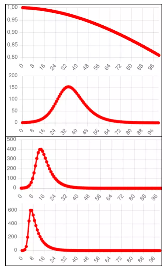
Note that the higher the value of $\underline{R}_0$, the higher the peak number of infections and the longer the epidemic's tail, rendering the curve less and less like the standard normal curve.
$\underline{R}_0$ can be generalised to $\underline{R}_t$, the average number of people infected by an infected person on a specific time step $t$. Given $\underline{R}_0$ and $s$, the proportion of the total population that remains susceptible, we have the following equation:
\begin{equation} \underline{R}_t = s \underline{R}_0 \end{equation}
The salient feature of $\underline{R}_t$ is that if it's below 1 the number of new cases is declining and if it's above 1 the number of new cases is increasing.
A slight misconception during the height of the Covid pandemic was to ascribe this feature to $\underline{R}_0$, instead of $\underline{R}_t$, but if $\underline{R}_0$ was below 1 there would have been no Covid pandemic. (I say "slight", because while people used the term $\underline{R}_0$, it was usually obvious in context that they were talking about $\underline{R}_t$ and such minor reductions in accuracy for the sake of simplicity are forgivable when explaining complex topics to the public.)
A more serious misconception during the height of the pandemic was the concept of herd immunity. Many implied that once herd immunity was reached, that was pretty much the end of the epidemic. But putting aside that the SARS-CoV-2 virus keeps mutating, with the consequence that recovered or vaccinated people become susceptible again, even in its idealised meaning herd immunity does not imply an epidemic has ended, or is even necessarily close to the end.
The Herd Immunity Threshold is simply the peak of the above graphs. It is the proportion of the population which is immune when the number of new infections begins to decline, or when $\underline{R}_t$ goes below one, and is given by this equation:
\begin{equation} 1 - {1 \over \underline{R}_0} \end{equation}
Related to this is the proportion of the population that remains susceptible when $\underline{R}_t$ goes below one. This is simply the second term in the Herd Immunity Threshhold equation:
\begin{equation} 1 \over \underline{R}_0 \end{equation}
The Herd Immunity Threshold is the proportion of the population that needs to be immune, either naturally or due to vaccination, to prevent a new outbreak of a disease. It is the target proportion of the population that vaccination programmes aim to reach to suppress an infectious disease, such as measles for example. Measles, mumps and rubella are examples of diseases which confer almost 100% immunity after recovery or vaccination (Vynnycky and White). But when a virus mutates as fast as Covid, Herd Immunity Threshold is a much less useful concept.
A problem with $\underline{R}_0$ and $\underline{R}_t$ is that they are easy to define and calculate in our idealised SIR model. They are hard to calculate in micro models or even complex macro models. And they are extremely hard to estimate in real world epidemics, which usually progress in fits and starts and not the nice smooth curves of our macro models. The is also true of the Herd Immunity Threshold.
Let's get a bit more complicated. We change our model world so that there's an Exposed compartment before an infectious one. When exposed a person is infected, but not infectious. In our model world the average exposure period is two days. This is an SEIR model.
We need to introduce a new parameter, $F$, the average number of days in the exposed compartment. Then $f = 1/F$ is the rate at which people move from the exposure to the infectious compartments.

Here are the difference equations:
\begin{equation} S_{t+1} = S_t - \beta I_t S_t \end{equation} \begin{equation} E_{t+1} = E_t + \beta I_t S_t - f I_t \end{equation} \begin{equation} I_{t+1} = I_t + f I_t - r I_t \end{equation} \begin{equation} R_{t+1} = R_t + r I_t \end{equation}
Here's the macro model version of SEIR using difference equations:
Here are the differential equations for the SEIR model:
\begin{equation} \frac{dS}{dt} = -\beta I(t) S(t) \end{equation} \begin{equation} \frac{dE}{dt} = \beta I(t) S(t) - f I(t) \end{equation} \begin{equation} \frac{dI}{dt} = (f - r) I(t) \end{equation} \begin{equation} \frac{dR}{dt} = r I(t) \end{equation}
Here's the macro model version of SEIR using differential equations:
Here's the micro model version of SEIR which attempts to match the difference equation macro model as closely as possible.
I ran the difference equation macro model once and the micro model 1,000 times with the number of initial exposures set to 1, 10, 50 and 100, and the initial susceptibles equal to 999, 990, 950 and 900 respectively.
Below are the results. As usual, because the micro model is stochastic, your results will probably differ a little.
| Macro model (difference eq) |
Micro model (1000 simulations) |
|||
|---|---|---|---|---|
| Exposed at start | Infections | Mean | Min | Max |
| 1 | 796 | 382 | 1 | 856 |
| 10 | 808 | 803 | 28 | 879 |
| 50 | 822 | 819 | 729 | 891 |
| 100 | 838 | 837 | 736 | 915 |
The results are consistent with what we see for the SIR models.
Measles is an interesting but frustrating infectious disease to model. It shows that the story of infectious diseases can often be more complicated than the approximately normal curve trajectory that William Farr posited.
This graph shows the oscillating nature of measles in England and Wales from 1950 to 1979. It is copied from Fine and Clarkson, 1982 (full paper on Sci-hub). Note how the epidemic returns approximately every two years. The arrow shows when the national measles vaccination programme was introduced, resulting in much smaller epidemics in subsequent years.
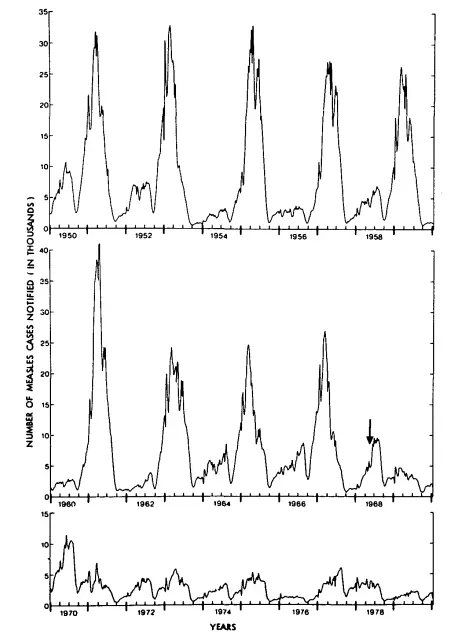
As Fine and Clarkson explained, there were two theories to try and explain this. One was that the measles virus mutated over time, with a consequent decline in immunity and resurrection of the epidemic. The other, now more accepted theory — but not without controversy because the data doesn't fit either theory as well as epidemiologists would like — is that never-before infected children entering schools provide a new susceptible population for the epidemic to spike. In between spikes, there are still measles cases, but in such low numbers that they largely go undetected.
Fine and Clarkson presented a set of difference equations, very similar to the SIR model. (Brian Williams has published useful slides explaining various models, including this model.) I've implemented a model only superficially different to theirs.
Our model world is a school with a thousand children. There are five grades so turnover is about 20% a year. We will assume the infectious period with measles is about two weeks (this isn't accurate but good enough for our over-simplified purposes), and this is our time-step. We set $\underline{R}_0$ to 2.
In our model that implements this model world there are just three compartments: $S$, $I$ and $R$. $N$ is the constant population size ($S+I+R$) and $\beta$ is the population turnover rate. We also assume people stay infected for exactly one time step. Here are the difference equations: \begin{equation} I_{t+1} = \underline{R}_0 I_t {S_t \over N} \end{equation} \begin{equation} S_{t+1} = S_t - I_{t+1} + \beta N \end{equation} \begin{equation} R_{t+1} = R_t + I_t - \beta N \end{equation}
This is a simple model but it's also unstable. Set $\underline{R}_0$ a bit high and either $S$ or $R$ drop below zero and the model falls apart. So I've slightly adapted the code for the above equations to not reduce $S$ or $R$ below zero. This keeps the model stable.
Notice the oscillations in measles cases every two or so years generated by the model. Adjust the value of $\beta$ and rerun the model to see how the oscillation period changes.It may be easier to view this graph by clicking on S and R in the graph legend, thus switching them off.
Also compare how different values of $\beta$ and $\underline{R}_0$ affect the oscillation period and peak number of infections.
On the face of it, this appears to capture the dynamics of measles epidemics. But here is a nearly equivalent micro model version.
Notice how the epidemic disappears. This is because in the macro model, which uses continuous variables, the number of infections never quite gets to zero, so equation 17 is always a positive number, albeit often a very tiny one. This means the epidemic will eventually resurrect in the macro model. But infection in the micro model is an all or nothing discrete affair. An agent is either infected or not. Quite quickly, the number of infections declines to exactly zero, and the epidemic cannot resurrect itself.
I've addressed this by creating a parameter, $r$, or Random Infections, that specifies the probability of randomly infecting an agent on each iteration. Try running the model with different values for this parameter. The length of the period between epidemic peaks is determined by it.
Do these models capture the dynamics of the real-world situation or do we simply have a set of equations (or rules in the micro model) that happen to approximate the infection distribution of measles? Where, for instance, did all the measles go in the non-epidemic years? I don't know the answer, and the models don't tell us. Another problem is that estimates of $\underline{R}_0$ for measles outbreaks are 12 to 18 (Vynnycky and White), much higher than 2, which we've used here.
Consequently, I find the models of measles here unsatisfying. Perhaps a better model is presented by Earn et al. published in 2000 in Science. They write: "It has been noted that annual cycles of measles epidemics occur in places where the birth rate is high (7). However, models normally take the average birth rate to be constant, implicitly ignoring the possibility that slow changes in this parameter could be a major driving force for dynamical transitions."
The 1918/19 global flu pandemic was one of the worst in history. The table below shows recorded deaths in India's Bombay Presidency.
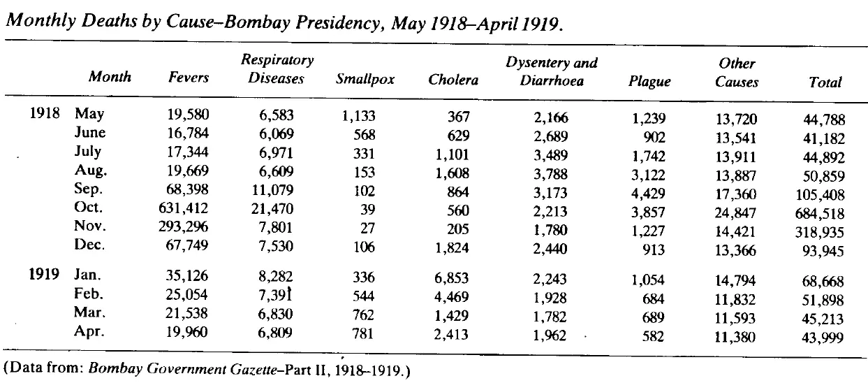
This table is astonishing. First, the scale of death is hard to comprehend. If we assume the background death rate before the influenza struck in August 1918 was the average of May to July 1918 then the number of recorded deaths due to the epidemic was well over 1 million, most of those in just two months, October and November.
Second, in 1918 the civil service — despite being hit by this massive disaster, as well as a world war that was already straining the Indian and British populations — was able to maintain death records with a completion rate that is still better than many countries in 2023. (Incidentally, the wave that struck Bombay in August 1918 was, according to Mills, the second one. The first struck in June. It's unclear to me whether the absence of a spike in mortality in June and July is due to delayed reporting of deaths or that the first wave was not especially virulent, or some other reason.)
Certainly no previous pandemic was chronicled in such quantitative depth. And yet estimating the number of global or even Indian deaths from the flu pandemic is hard and controversial. They range from fewer than 20 million to over 100 million, none totally implausible. (My own bias is towards the lower end of the scale.)
Let's do some crude calculations:
This is implausible. The Bombay Presidency is not a representative sample of what happened on average. Bombay was hit especially hard by the pandemic. Besides being overcrowded and people living in ghastly conditions, Bombay's docks served as a port for World War I soldiers. This traffic was quite possibly one of the main drivers of the epidemic. If anything, this shows that one must beware of crude calculations of pandemic deaths.
There have been much more sophisticated efforts. Spreeuwenberg et al. (2018) write:
"The [global death] burden [of the 1918/19 influenza pandemic] has been estimated many times over the past 100 years, and the estimated burden gradually has increased. One of the oldest estimates was made by Jordan in 1927, who estimated the global burden to be approximately 21.6 million deaths. Patterson and Pyle, in 1991, estimated the burden to be 30 million (ranging from 24.7 million to 39.3 million). In 2002, Johnson and Mueller reported a range of 50 million to 100 million deaths, with 50 million closer to the results from the studies they cited, and 100 million being the upper limit, because they believed 50 million to be an underestimate."
Spreeuwenberg et al. estimate just over 17 million deaths and not more than 25 million. "Our results suggest the global death impact of the 1918 pandemic was important but not as severe as most frequently cited estimates," they write.
Estimating the number of deaths is difficult enough; estimating the number of infections is very much harder. And how does one even begin to estimate $\underline{R}_0$ with such imperfect data and such wide disagreement? The point here is not to weigh into this debate which would require considerable study and expertise. Rather it is to show how imperfect our knowledge is of the spread and number of deaths brought by infectious diseases.
This remains true of epidemics today. The Economist has been attempting to estimate the number of excess deaths caused by Covid globally. As of 28 February 2023, the authors state: "We find that there is a 95% chance that the true value lies between 16.5m and 27.2m additional deaths." Besides being a wide range of the number of deaths of the most documented and studied pandemic in history, one is struck, when delving into their analysis, by the poor quality of data from many countries.
If we compare The Economist analysis to the lower bound 1918 flu mortality estimates, it is possible that Covid may have killed more people. But the global population is about four times greater now and, also, the age distribution of Covid deaths was very much older than the flu pandemic. That the death tolls from the 1918/19 influenze pandemic and Covid are catastrophically high is indisputable. But precise estimates should be treated with great caution. The same can be said for the Antonine Plague (165-180AD), the Justinian Plague (541-549AD), the Black Death (1346-1353), smallpox through the aeons, tuberculosis through the millenia, HIV over the past 40 years, and a whole bunch of other infectious maladies. Modellers should be modest.
In the late 2000s until 2015 there was a feisty discussion in the HIV field about the optimal time for people with HIV to start antiretroviral treatment. These pills, taken daily for life, reduce the number of HIV virions in the blood of people with this infection, usually to undetectable levels. This brings two advantages: (1) it extends life-expectancy to almost normal and (2) it reduces the risk of transmitting the virus to others, though this was not known with much confidence until a large clinical trial confirmed it in 2011.
The ideal time to start treatment wasn't clear because of three concerns: (1) the side effects of the drugs, (2) if drug resistance developed quickly a person would lose the benefit of the drug regimen, so starting later might extend the period of drug efficacy longer, and (3) the cost of the drugs.
In 2015 the START trial showed that the benefit of starting treatment as soon as a person was diagnosed was substantial. Moreover drug resistance and serious side effects with newer antiretroviral regimens have become minor problems. Nowadays medical guidelines recommend that people with HIV should start treatment when they are diagnosed; no need to wait.
Nevertheless in the late 2000s all of this was unclear. World Health Organisation researchers (Granich et al. 2009) published models in The Lancet that showed that a policy of actively testing and immediately treating people with HIV in South Africa, the country with the most number of people with this virus, would reduce its HIV prevalence to a negligible level in 50 years.
The paper certainly made a splash, evoking vociferous discussion. According to Google Scholar it has been cited over 2,300 times. I suspect that until the Covid pandemic it was the most cited infectious disease model.
The graphic below from The Lancet paper describes one of their models.
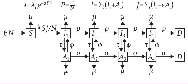
This is a much more complex model than our SEIR or measles ones. It accounts for population growth and deaths. The model specification has 10 compartments and another 10 parameters. Here is a macro model (using difference equations) implementation of Granich et al.
In the results table, the total number of infections (the sum of compartments I1 through I4 and A1 through A4) is tracked in the column with the heading I. Try adjusting the parameters, especially τ, and rerunning the model to see how the course of the epidemic changes, particularly the S (susceptibles), D (deaths) and I (infections) columns. For example set τ to 0.00 (in other words no treatment takes place) and notice how the population declines, and infections and deaths skyrocket.
We can quite easily implement a micro model of this.
| Macro | Micro | |||||
|---|---|---|---|---|---|---|
| τ | Susc. | Inf. | Dead | Susc. | Inf. | Dead |
| 0 | 724 | 477 | 374 | 681 | 365 | 470 |
| 0.15 | 1165 | 279 | 116 | 1145 | 122 | 281 |
| 0.3 | 1194 | 268 | 94 | 1188 | 96 | 269 |
While I have done my best to match the two models, the course of the epidemic is now highly non-linear and I haven't achieved near-perfect matching like in the SIR and SEIR models. Sometimes in infectious disease modelling this is fine; we merely hope for plausible approximations and the differences between the outputs of the two models may then be inconsequential. But sometimes more precise estimates are required and if a macro and micro model making similar assumptions give different outputs then the task of explaining why becomes important.
In March 2020 – a few months after the appearance of the Covid pandemic — a micro model by Neil Ferguson and his team at Imperial College in the UK was widely reported in the media. The modellers considered how various interventions, such as isolation, quarantining, social distancing and school and university closures would affect the spread of SARS-CoV-2 and the pressure on hospitals.
Their report is detailed and nuanced. There is extensive discussion about mitigating the effects of Covid — reducing $\underline{R}_t$ but not below 1 — versus suppressing it completely — reducing $\underline{R}_t$ below 1. It also had to make a plethora of assumptions given how little was understood about Covid at the time.
Unsurprisingly, as with any model that tries to predict the future, it got some things wrong, such as the time period over which Covid would peak. It also didn’t consider that SARS-CoV-2 would mutate and that the epidemic would return in waves of differing infectiousness and virulence.
The report concludes that social distancing would have the largest impact. Combining this with isolating infected people and school and university closures may suppress transmission below the threshold of $\underline{R}_t = 1$, the authors wrote.
They also pointed out that, “to avoid a rebound in transmission”, these policies would need to be maintained until large stocks of vaccine became available. They pessimistically predicted this would be 18 months or more, but in fact vaccines became available near the end of 2020, although most countries wouldn’t start rolling them out until 2021.
The authors recommended using hospital surveillance to switch these measures on and off. Importantly they wrote: “Given local epidemics are not perfectly synchronised, local policies are also more efficient and can achieve comparable levels of suppression to national policies while being in force for a slightly smaller proportion of the time.”
They were cautious:
"However, there are very large uncertainties around the transmission of this virus, the likely effectiveness of different policies and the extent to which the population spontaneously adopts risk reducing behaviours. This means it is difficult to be definitive about the likely initial duration of measures which will be required, except that it will be several months. Future decisions on when and for how long to relax policies will need to be informed by ongoing surveillance."
They also considered mitigation instead of suppression:
"Our results show that the alternative relatively short-term (3-month) mitigation policy option might reduce deaths seen in the epidemic by up to half, and peak healthcare demand by two-thirds. The combination of case isolation, household quarantine and social distancing of those at higher risk of severe outcomes (older individuals and those with other underlying health conditions) are the most effective policy combination for epidemic mitigation."
There is very little emphasis on actual results. The same is true for Imperial College's news summary of the report for the general public. This seems to be a sensible approach. No model in March 2020, fewer than three months after Covid had been discovered, could rely on sufficient accurate knowledge to predict the future with any realistic accuracy. Even when diseases are well-understood, and slow moving, like TB and HIV, it is very hard to predict future infections and mortality with much accuracy.
What models can do, and what the Imperial College model did, is show the approximate magnitude of certain interventions on mitigating or suppressing infectious outbreaks.
Yet the Imperial College model was widely criticised, especially by those with an ideology opposed to stringent government intervention.
In April 2020, the US-based Cato Institute lambasted the model. It criticised its pessimistic predictions, which hadn’t come close to being true by that time. "Neither the high infection rate nor the high fatality rate holds up under scrutiny.” The article, which echoed the Cato Institute’s opposition to lockdowns or any stringent government measures to control the epidemic, stated:
"The trouble with being too easily led by models is we can too easily be misled by models. Epidemic models may seem entirely different from economic models or climate models, but they all make terrible forecasts if filled with wrong assumptions and parameters.”
Much is made of the model’s estimate of 2.2 million Covid-19 deaths in the US in the absence of any interventions, something the modelling report correctly did not emphasise at all.
The critique is not entirely unfair: it makes the point that the model and the response of governments didn’t account for some people voluntarily taking action to reduce their risk of infection. And the long-term repurcussions of closing schools and universities for long periods of time are still being debated, and felt.
But much of the Imperial College model did in fact stand up to scrutiny in the long run. There have been over 1.1 million Covid deaths in the US. At least one study estimated that vaccines saved over a million lives. This suggests that Covid in the US, left unchecked, may well have claimed about 2 million lives. But the Imperial College model did not get the timeframe or wavy nature of the pandemic right.
Even so, this is not the point. The modellers didn’t emphasise the precision of their measurements. That wasn’t the aim of their model. Instead they reached broad conclusions, the main one being that if the pandemic was left unmitigated or unsuppressed it would have a much more devastating impact. On this the modellers were right.
In South Africa the earliest released government model was widely criticised by opponents of lockdowns, who wanted to minimise the pandemic’s effects to support their arguments. The model had a quickly done rough calculation feel to it. Like the Imperial College model it didn’t account for mutations and the consequent wavy nature of the disease, and it also predicted a much swifter unfolding of things. But, frankly, given the state of knowledge at the time, a simple SIR-type model was arguably sufficient to make the point that reducing social contacts would slow the pandemic.
Given the heated ideological disputes in response to Covid, perhaps there was no way early modellers could have escaped criticism, even if they had miraculously estimated the trajectory of the pandemic with pinpoint accuracy. Nevertheless modellers might consider explicitly explaining upfront that it is the broad conclusions rather than the specific estimates of their model that are important.
Also, when an epidemic’s parameters are hard to know with precision or vary a lot from place to place, modellers should perhaps consider running thousands of simulations that randomly perturb the parameters within reasonable ranges. Then we can present multiple possible scenarios to the public. Though this must be done in a way that emphasises the more likely scenarios and that does not overwhelm the public with a plethora of possibilities. Done properly, I hope this acknowledgement of our ignorance may actually gain greater public confidence in the modelling process.
But we should also not be naive. No matter what honest modellers do, their work will be distorted by those whose politics are inconsistent with the model's conclusions. And predictions that turn out to be incorrect will be pounced on.
Since the 1990s models to predict the trajectory of the HIV epidemic in South Africa have been useful for estimating medical need and cost. The most widely acclaimed of these was the Actuarial Society of South Africa model, predominantly developed by Rob Dorrington. This was enhanced, mainly by Leigh Johnson into what is now the Thembisa model.The full citations for the model are: Johnson LF, May MT, Dorrington RE, Cornell M, Boulle A, Egger M and Davies MA. (2017) Estimating the impact of antiretroviral treatment on adult mortality trends in South Africa: a mathematical modelling study. PLoS Medicine. 14(12): e1002468. and Johnson LF, Dorrington RE, Moolla H. (2017) Progress towards the 2020 targets for HIV diagnosis and antiretroviral treatment in South Africa. Southern African Journal of HIV Medicine.18(1): a694
The Thembisa model is extremely complex and carefully calibrated to match known data points. It uses a monthly time step and produces a huge number of outputs, including the South African population size, number of deaths, number of deaths from HIV, the number of people with HIV, the number of new infections and more. This is all broken down by age group and sex. Thembisa includes several interventions including antiretroviral treatment, male medical circumcision, pre-exposure prophylaxis and the prevention of mother-to-child transmission.
South Africa's latest available census results are from 2011. A census was conducted in 2022 but has not yet been published (and there are concerns about how well the census was conducted). Because the census data is so old I (and others) use the population size, life expectancy and other demographic outputs of Thembisa when writing about these things. The model, which is meticulously constructed, has de facto become the definitive source of population estimates. This is despite my cautions about using models to predict the future accurately. But it's justified in this case because (1) the dynamics of HIV are currently still better understood than Covid and the epidemic fluctuates at a stately pace compared to Covid, and (2) the Thembisa model has decades of careful work behind it.
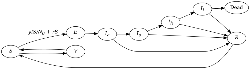
Here is a model world that tries to capture the nature of a Covid outbreak in a small community:
In our model, our compartments are $S$, $E$, $I_a$, $I_s$, $I_h$, $I_i$, $R$, $V$ and $D$. The time step is one day. The rate at which people transition between two compartments is specified by the name of the source compartment, an underscore, _, and the name of the destination department. For example if we set $I_a\_I_s$ to 0.2, this means there is a 20% chance that people in the infectious asymptomatic compartment will move to the infectious symptomatic compartment on a time step.
People in some compartments can transition to one of two mutually exclusive compartments. For example there is also an $Ia\_R$ transition, representing people who move straight from asymptomatic infection to recovery. The model must first calculate the one transition and then the other. The order matters. The order in which the transitions are listed in the models below is the order in which they are calculated.
It's tricky to use $\underline{R}_0$ directly to calculate the number of people that become exposed per time step in this model. This is because the average number of days of infectiousness, $D$ in equation \eqref{eq:R0}, is very hard to calculate. Instead the parameter $y$ replaces it so that on a given time step the number of new infections (i.e. the transition from $S$ to $E$, $S\_E$) is: \begin{equation} S\_E = { {y \times I \times S} \over N_0 } \end{equation} where $N_0$ is the initial population.
$I$ is calculated by multiplying the infectiousness of each infectious compartment by the value of the compartment itself and then summing these:
\begin{equation} I = I_{I_a} I_a + I_{I_s} I_s + I_{I_h} I_h + I_{I_i} I_i \end{equation}
The rate at which susceptible people are exposed outside the community on a time step is given by the parameter $r$.
Here is our macro model using difference equations.
Here is a micro model that attempts to match the macro model as much as possible.
Try experimenting with different parameter values. In particular, in the default setting, we have a very vaccination-averse population. See what happens to the infections and deaths if a much higher vaccination rate is used.
There are many shortcomings of these two models. Here are a few:
Frankly with the default settings, neither model's infection curve looks much like any I've seen, and this may very well be due to these shortcomings.
Removing these shortcomings would be easier in a micro model than a macro one. The number of compartments would multiply rapidly and the resulting complexity of the macro model would likely tax even highly competent programmers. Heterogeneity is often especially hard to capture in macro models.
Models can be used to show the public why a medical intervention is useful. For example, here is a straightforward model that shows that if infectious people isolate during the outbreak of an airborne disease, the epidemic can be slowed down (we "flatten the curve" — in particular the red one representing the number of infections — to use a phrase that became popular during Covid). The agents move somewhat randomly. A susceptible agent becomes infected if it touches an infectious one, with a probability determined by the Risk infection parameter, which defaults to 1.
In the first version of the model, no one isolates.
In the second version infectious agents are likely to isolate for most of the the period of their isolation. When agents isolate they are moved into the left section of the Population panel and they remain stationary for the duration of their isolation. They may recover in that period. The models are identical except that the isolation time steps parameter is set to 0 in the top model.
The models are abstract but also simple. Unlike our other models, a time step here doesn't correspond to a day, but to all the non-isolated agents moving one pixel. The model is stochastic so results will differ across runs for the same parameter values. Occasionally a run of the second model will result in more infections than a run of the first one. Adjust the parameters to see how the average level of isolation adherence affects the number of infections, or how the efficacy of isolation differs depending on the disease duration and level of infectiousness.
A rather different type of model to the ones we've discussed are maps that trace the source and spread of an epidemic. John Snow famously did the first such map to trace the outbreak of the 1854 cholera epidemic in London to a public water pump on Broad Street in Soho.
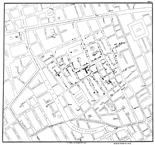
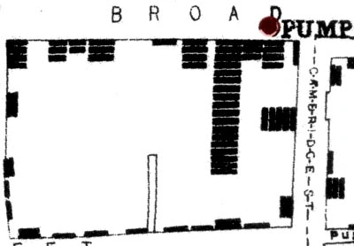
Each bar represents a cholera death in a household. Note how the deaths cluster around the Broad Street pump. At the time it was believed that cholera was caused by particles in the air caused by decomposition. Snow overturned this theory by showing that the source of infection was in the water from the public pump that households in the area used. The full story is more complicated and fascinating and told fantastically well in The Ghost Map by Steven Johnson.
More recently, in July 2022, Michael Worobey and his colleagues showed that the likely origin of Covid in humans was the Huanan Seafood Wholesale Market. They presented several strands of evidence. One of the most convincing is this map which also shows how early cases clustered near the market:
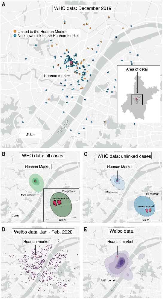
"(A) Locations of the 155 cases that we extracted from the WHO mission report. Inset: map of Wuhan with the December 2019 cases indicated with gray dots (no cases are obscured by the inset). In both the inset and the main panel, the location of the Huanan market is indicated with a red square. (B) Probability density contours reconstructed by a kernel density estimate using all 155 COVID-19 cases locations from December 2019. The highest density 50% contour marked is the area for which cases drawn from the probability distribution are as likely to lie inside as outside. Also shown are the highest density 25%, 10%, 5%, and 1% contours. Inset: expanded view and the highest density 1% probability density contour. (C) Probability density contours reconstructed using the 120 COVID-19 cases locations from December 2019 that were unlinked to the Huanan market. (D) Locations of 737 COVID-19 cases from Weibo data dating to January–February 2020. (E) The same highest probability density contours (50% through 1%) as shown in (B) and (C) for 737 COVID-19 case locations from Weibo data."Source: Worobey et al. 2022. The Huanan Seafood Wholesale Market in Wuhan was the early epicenter of the COVID-19 pandemic. Science Vol. 377, No. 6609. See also: Pekar et al. 2022. The molecular epidemiology of multiple zoonotic origins of SARS-CoV-2. Science Vol. 377, No. 6609, and Jang and Wang, 2022. Wildlife trade is likely the source of SARS-CoV-2. Science Vol. 377, No. 6609.
While at the time of writing there is still some speculation that SARS-CoV-2, the cause of Covid-19, may have leaked from a laboratory in Wuhan, there is no compelling evidence that this is the case. Instead supported by the above analysis and molecular analysis of the early cases, Worobey et al. conclude: "The precise events surrounding virus spillover will always be clouded, but all of the circumstantial evidence so far points to more than one zoonotic event occurring in Huanan market in Wuhan, China, likely during November–December 2019."
The case for the Huanan market being the place where the first humans were infected with SARS-CoV-2 was strengthened by the discovery of animal DNA and RNA, particularly raccoon dog, in samples that had been swabbed in the market and that tested positive for virus. This doesn't conclusively prove that there were live infected animals in the market and that they transmitted the virus to humans, but it adds to the circumstantial evidence.
There is much dispute, mainly on social media and by some departments in the US government, on the origins of SARS-CoV-2. But in science, and perhaps in most things, it makes sense to go with where the current evidence points. While this maxim isn't always straightforward to apply, here it appears to be. As things stand, the origins of SARS-CoV-2 were likely between animals and humans in a wet market, not in a laboratory.
Imagine there's an outbreak of a new infectious disease in a distant part of the world. Luckily scientists quickly develop a test for the infection. Then the disease lands in your city, where you are the head of public health. You organise for 1,000 people to be randomly tested daily. Using this, you have the daily infection rate in your city. Now you want to fit an SEIR model to your data, so that you can predict the future trajectory of the epidemic.
In the graph below, the blue line is the daily number of infections — the observed values — in the sample of 1,000 people. The pink line represents the predicted number of infections by an SEIR model. Adjust the values of the parameters — (1) $\underline{R}_0$, (2) average number of days in the exposure compartment, and (3) average number of days in the infectious compartment — until the predicted values fit the observed data as closely as possible. (The observed values change every time this webpage is refreshed or you click the New observations button, so if they look especially terrible, simply refresh the page or click the button. Also, very occasionally, the web page will load with the model already calibrated. In which case, simply reload the page.)
What you've just done is calibrate a model. Of course the real world is never as neat and tidy as this. (1) Daily surveys like this can almost never be done. (2) Even if they could the sample size would not consistently be 1,000. (3) This is coded so that the observed values are always within 5% of the points along an SEIR model with integer values for the three parameters in a homogenous population; good luck finding a real-world epidemic that's so accommodating.
When building a model that tries to explain the nature of a real epidemic, especially if it tries to predict the future course of that epidemic, it will likely be important to calibrate the model against known data points.
For example the Thembisa model is calibrated to fit adult HIV prevalence, antiretroviral metabolite data and adult mortality up to particular years. The model then produces a bunch of inferred demographic outputs up to those particular years, and also projects into the future. It's a complex model and the calibration process is especially complicated and worth reading.
The topic of model calibration (which, for the most part, is another name for function optimization, function approximation or regression analysis) could do with much more exposition in modelling literature. This is a somewhat superficial introduction.
The first thing needed to calibrate a model is a way to measure the error between the real world calibration points and the model's outputs. The mean squared error (the MSE value in the graph above) is often a good choice for such an error function. Given $n$ known real-world data points $Y_0, Y_1 ... Y_n$ and model outputs $y_0, y_1 ... y_n$, the mean squared error, $E$ is: \begin{equation} {1 \over n} \sum_{1}^{n} {(Y_i - y_i)}^2 \end{equation}
Formally, the goal of calibration then is to find a set of values for the model parameters, $p_1, p_2 ... p_m$, that minimises the error function. (If you have come across the term sum of the squared residuals, the mean squared error is the same thing divided by $n$.)
Calibration of complex models can involve thousands of model executions. Stochastic micro models will generally take much longer to calibrate than their equivalent deterministic macro ones. There are two reasons for this: they take longer to run and, because they are stochastic, the model may need to be rerun multiple times with each set of parameter values, $p_1, p_2 ... p_m$, and then $y_1, y_2 ... y_n$ will be the average output values across the runs. This is because a single run, or even only a few runs, may produce outputs that are far from the mean for that particular set of parameters.
There are many error minimization techniques. Here are brief descriptions of a few:
I've tried to implement the micro models to match as closely as possible the macro models that use difference equations. The code makes certain compromises to do this. For example, $\lambda_t$ is calculated using the number of infections at the end of the previous time step, not the current number of infections which may have changed as the infection event iterates over agents. Other than for the purpose of trying to match the models as closely as possible, I see no reason to do this.
Moreover, while thinking in terms of compartments make sense for macro models, for micro, or agent-based, models, it's more natural to think of agents having states, rather than being in compartments. In a macro model if you wish to include additional characteristics such as sex and age group, you would need to replicate all the compartments for each sex and age group. But in a micro model, without compartments, an agent could have a sex, age and state. A state may even be partial (e.g. an agent transitioning from an asymptomatic to symptomatic phase — with different levels of infectiousness or different subsequent behaviours — may do so gradually), or an agent may be in multiple states. As models increase in complexity, macro models become extremely difficult to implement, while the increase in programming complexity in micro models is much slower.
Nevertheless in the micro models here I continue to talk of agents being in compartments rather than states, simply to keep the nomenclature consistent with the macro models.
There is far more debate on the Internet about which are the best programming languages than the topic deserves. In fact, there are many good programming languages and all of them are flawed. Write your first simulations in a programming language you feel comfortable with. If it's a prototype it doesn't matter if it's Python, R, Ruby, Basic or whatever your favourite algebra for expressing algorithms is.
If you need your simulation to execute many thousands of times and you are finding it too slow, changing to a compiled language like C, C++, Go, Fortran, Rust, Java or even a lisp-type language, may be necessary. But often the cause of execution being too slow isn't the language but an algorithm you might be using. Perhaps consider optimising or improving an algorithm before going to the effort of learning a new programming language.
For what it's worth I tend to implement my micro models in Python when I'm just prototyping and then C or C++ if I truly need a lot more speed. But the models on this web page are implemented in Javascript, because that is the main programming language that the most popular web browsers support.
During Covid, there was much consideration of the effectiveness of isolating infected people and quarantining their contacts. (From hereon, for the purposes of this discussion, the word isolation refers to both isolating and quarantining.) A question that arose from this is for what kinds of airborne infectious diseases is contact tracing coupled with isolation likely to be effective?
To answer this question we simulated thousands of infectious diseases. Each simulation had 10,000 agents and ran for 500 time steps. Each disease was defined by randomly peturbing a number of parameters within specified ranges. We generated 15,000 diseases. For each disease we compared five different scenarios, ranging from no isolation at all to complete adherence to isolation of infectious people and their contacts. Because this was a stochastic microsimulation, we ran each model ten times to get an average for the model's outputs. In total we ran 750,000 simulations (Geffen and Low, 2020). In fact, since we had several test runs, as well as bugs and flops along the way to our final set of results, we actually ran millions of simulations.
It would be impractical to have done this using an interpreted language like Python or R. It would have been far too slow. Instead we coded it in C++.
Modellers I've spoken to often yearn to make their micro, or agent-based, models much faster. They usually don't have a computer science background and only know a smattering of C or C++. If you are in this boat, below is a heavily commented non-trivial, but not too complicated ether, example model in C++ that can be extended quite easily. (In the Github repository it is model_example.cc.) And if you've got some experience with Python, to make it easier to understand the C++ exampled, I've coded an almost equivalent Python version of the program. (In the Github repository it is model_example.py.)
The model has these characteristics:
Here is the code:
Thanks to Alex Welte for advice, and Leigh Johnson, Juliet
Pulliam and Stefan Scholz for suggesting several improvements. I
have learnt much about the modelling done here through discussions
with them as well as Marcus Low and Eduard Grebe. Stefan advised
me, introduced me to various modelling software tools and helped me
to understand calibration better.
All errors are my
responsibility.